Previously, I talked about Bayesian statistics. This will be a continuation of that post, based on yet another topic I’ve tried to learn on my own. The only difference is that we’re spicing up the title with alliteration and switching up the theme: this post will be centered around Halloween, so get ready for some spooky music and literature (costumes are optional).
Recall that we worked really hard to show that a beta prior could account for a fair range of beliefs and had a nice analytical solution (i.e. it was possible to integrate that pesky denominator). Unfortunately, even with this discovery, you don’t have to get too creative to come up with situations that we can’t adequately describe. For instance, what if we have a bimodal distribution? That is, say there’s a class where you expect a cluster of A’s, a group of C’s, and not much else in between. A beta distribution certainly can’t capture this “double hump”. Fortunately, we have a solution. Take a look at \(\text{Beta}(5, 5)\) (figure b) below. Note that we can discretize and approximate this distribution using 25 points (figure a), or however many you’d like.
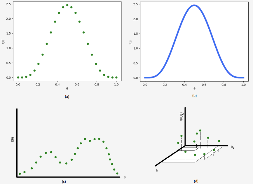 We can also “manually” tune the prior to our heart’s content and come up with some fun looking distributions such as figure c. Instead of integrating, we can simply sum up our evidence as follows:
You may be thinking, “Jeez, this is extremely tedious and I don’t want to add numbers,” in which case, I agree. That’s what computers are for!
At this point, it seems that all our problems are solved. Yet, like a bogus super supplement claiming to remedy all ailments, this is simply not true. In reality, life is complicated and we’re often dealing with more than one variable as shown in figure d. Let’s say you have 6 variables with 1000 discrete values for each. That’s already \(1000^6 = 10^{18}\) possibilities to evaluate!
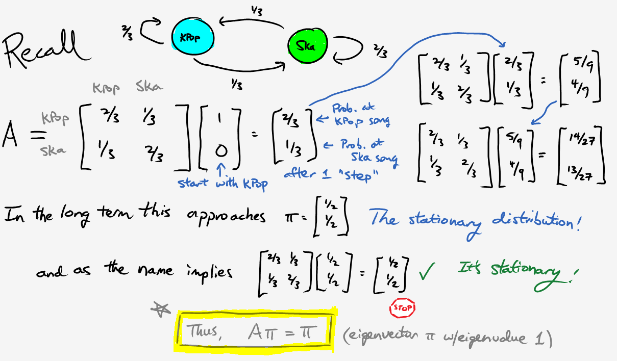
So, to break through the walls of intractability, it’s time to bring out the big guns: Markov chains.
Musical Markov Chains
Video questions:
If we start with a knight ♘ in the corner, how many hops would it take, on average, for it to return to its starting square?
168 hops (look at A1 in the stationary distribution at 9:40).
What if we start with a rook ♖ in the corner?
The rook can move to 14 different positions regardless of where it starts. Thus, the stationary distribution is 1/64 for all states, and so it will take 64 hops to return.
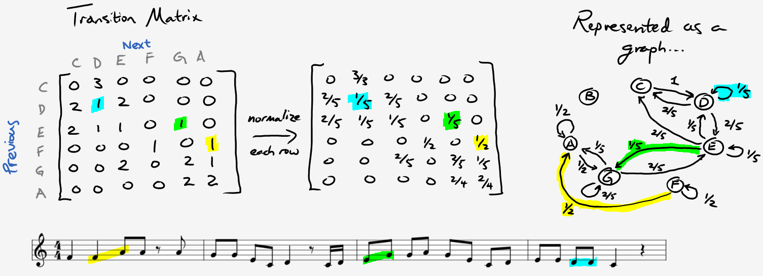
If you have some computer science background, a Markov chain is just a graph where nodes are states in the state space and edges refer to probabilities of transitioning from one state to another. To gain intuition with this idea, let’s compose some music. If you’re uncomfortable with musical notation, don’t fret, we’ll keep it basic. Just use this reference and take some time to memorize a few positions on the staff line. Afterwards, listen an excerpt from Oh Susanna by Stephen Foster:
One way we can create music is to simply count the frequency of each note, divide by the total number of notes, and then generate notes with those probabilities. In the case above, we would have:
| C | D | E | F | G | A | B |
| 4/25 | 5/25 | 5/25 | 2/25 | 5/25 | 4/25 | 0/25 |
Here’s a sample of our “zeroth-order” Oh Susanna spin-off:
This doesn’t really resemble our original tune, and even though it’s not terrible sounding, we could do better. The problem is that music typically follows some bigger patterns, but we’re just pulling random notes from the same key. Instead, what if we included some context by choosing the next note based on our memory of the previous one?
In other words, we’ll want to make a table with \(P(x_n | x_{n-1})\).
Here’s a “first-order” version of Oh Susanna:
Now that sounds a lot more like a “Foster-inspired” work! We could continue with second-order, where we would consider the last two notes and calculate \(P(x_n | x_{n-1}, x_{n-2})\), or third-order and so forth. However, do keep in mind that we’d eventually end up plagiarizing the entire piece, which we don’t want either. All right, time to test this out. I’ve written a short motif below. Perform a first-order Markov analysis for the top treble line only (ignore the bass; that was just for fun).
Once you’re done with that, it’s show time. First, listen to the piece below and note that the rhythmically-challenged soloist plays a drone (if it gets unbearably out-of-sync, try restarting). Next, stop the music and assign the transition probabilities (decimals) you just calculated by clicking on the appropriate arrow (the self-directed edge \(e_0\) is automatically calculated as \(1 - \sum_{\substack{e_n \in E_{out} \\ e_n \neq e_0}} e_n\) where \(E_{out}\) is the set of outgoing edges for a given vertex). Finally, enjoy your composition!
Solution:
AB: 1/2, AC: 1/2, BA: 3/5, BC: 2/5, CB: 3/8, CC: 1/8, CD: 2/8, CE: 2/8, DC: 3/4, DE: 1/4, EA: 1/3, ED: 2/3
To round out this discussion, Hiller and Isaacson used Markov chains to compose the fourth movement of the Illiac Suite. You can view their original publication, or read a bit more about their experiment in this summary. Lastly, I highly recommend Musimathics, which is the textbook I referenced for the “Oh Susanna” examples.
The Metropolis Algorithm
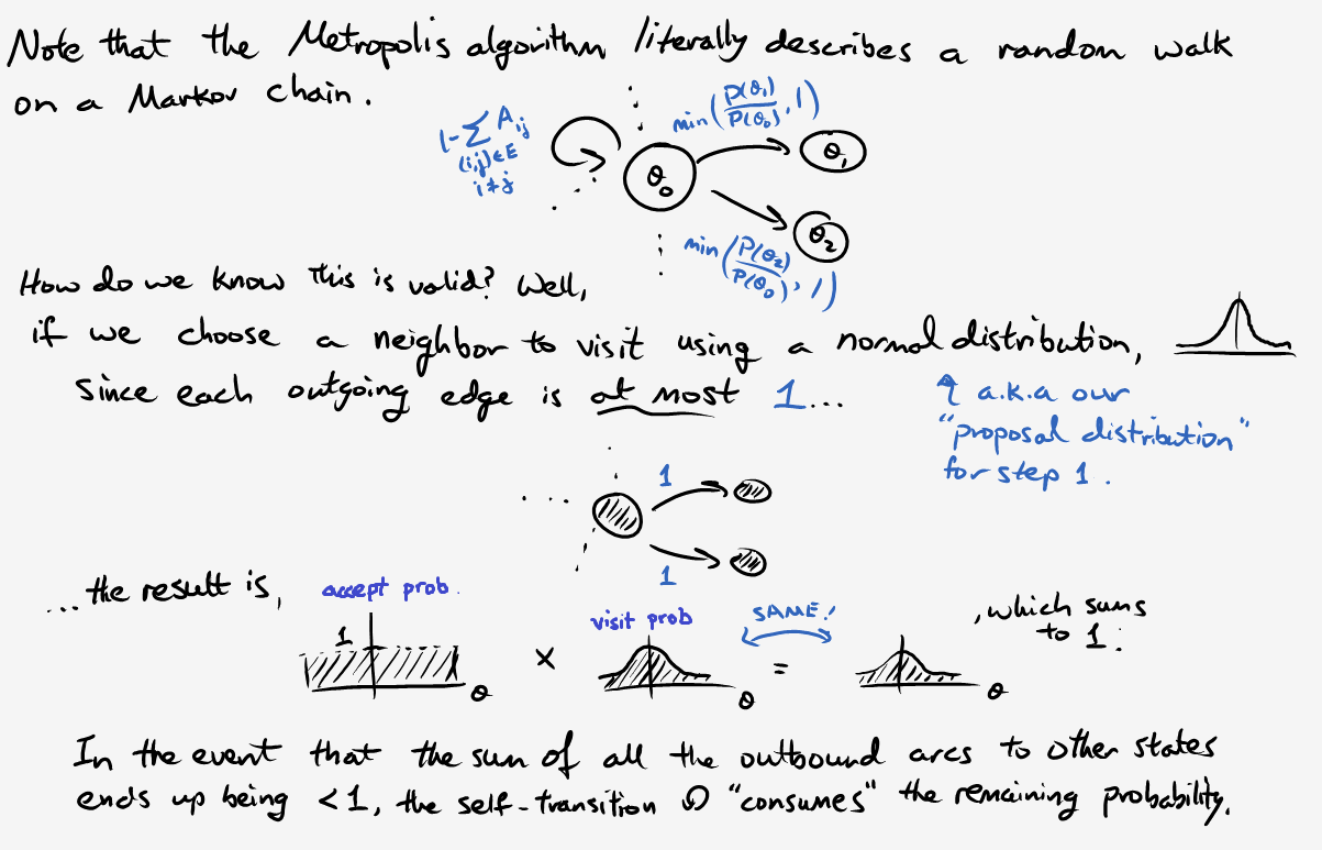
All right, now that we know what a Markov chain is, how does that help with our original problem? Simply put, we’re going to generate representative values from our posterior distribution by randomly walking around a Markov chain. Once we have a good sample, we can then estimate the mean, credible intervals, and other parameters using significantly less than one quintillion computations. Like any good “how-to” tutorial, our algorithm requires only three easy steps:
Given a starting point \(\theta_{current}\)…
Step 1: Propose a neighbor \(\theta_{prop}\) to visit in state space.
Step 2: If \(P(\theta_{prop}) > P(\theta_{current})\), go there!
Step 3: Otherwise, only move with probability \(P(\theta_{prop}) / P(\theta_{current})\).
Record the state and repeat as necessary.
We can condense steps 2 and 3 by defining the following “move” probability:
\[P_{move} = \min{\bigg( \frac{P(\theta_{prop})}{P(\theta_{curr})}, 1 \bigg)}.\]Note that we merely need to calculate the unnormalized posterior distribution \(P(\theta) \propto p(D \vert \theta)p(\theta)\). As long as the likelihood and prior are easy to compute, there’s no need to slog through the evidence \(p(D)\) (and yes, I realize the capital/lowercase notation is a tad confusing). At this point you might say, “This seems like voodoo magic; prove that it works.” Fair enough. Allow me to fill in some of the missing details:
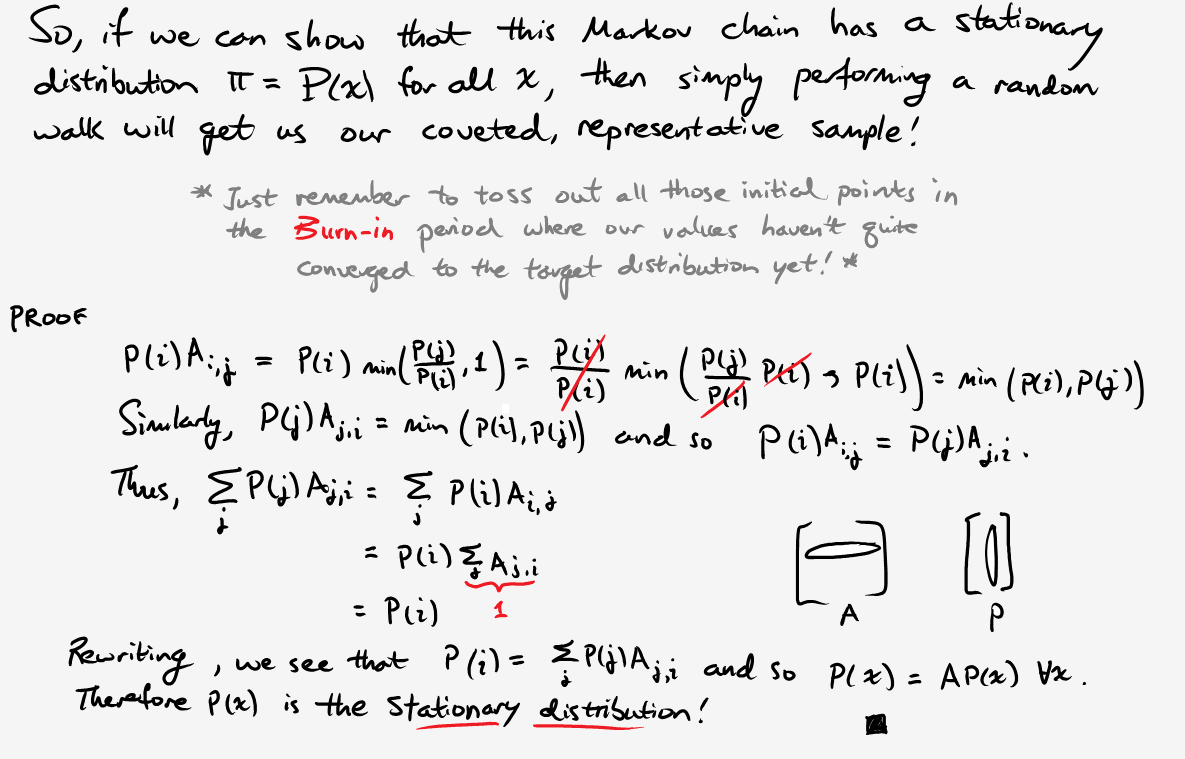
There are still a few open questions. For instance, how do we know there aren’t other stable states? How long does it take to converge? How do we know that this stationary distribution even exists? To answer these questions and more, here are some of the resources I used while trying to write this article: a blog entry, a pdf document (that discusses the section below), and this textbook with a bunch of dogs on the cover. Some of them are fairly technical, yet understandable with enough time and scratch paper.
Murder Mystery
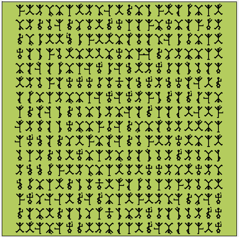
To wrap this up, here’s a fun application of the Metropolis algorithm. In the Sherlock Holmes short story “The Adventure of the Dancing Men”, a client hands him a piece of paper with the following figures:

Turns out, this is a substitution cipher where each stick figure represents a letter. Assuming we have one figure per letter, this would correspond to 26! permutations. Consequently, cracking the code with brute force is not a feasible option. Instead, let’s use the Metropolis algorithm. To get a matrix of transitions \(M\), we can use the same approach as the musical notes, but count letters from some English text (in this case, War and Peace). Our state space will be the set of mappings \(f\) from codes to letters. In order to select a neighbor, randomly transpose two symbols (making sure they’re not the same ones). Finally, we’ll compute a “plausibility” as follows:
\[P(f) = \prod_{i} M(f(x_i), f(x_{i+1}))\]As a quick side note, we run the risk of overflow and round-off errors since these values are going to quickly blow up. So in our actual implementation, we’ll use the log plausibility, which also allows us to replace repeated multiplication with addition.
\[\log{(P(f))} = \sum_{i} \log{(M(f(x_i), f(x_{i+1})))}\]The move probability then becomes
\[P_{move} = \min{\bigg(\exp{ (\log{P(\theta_{prop})} - \log{P(\theta_{curr})} }), 1 \bigg)}.\]The idea behind this definition is that if a mapping results in a decoded message with similar frequencies to our English reference text, then it’s probably the right one (or close to it). Important caveat: we don’t want an entire sample. Just keep track of the representative mapping that results in the highest plausibility score. Here’s an example with six letters. I ignored punctuation and then tallied in the usual fashion.
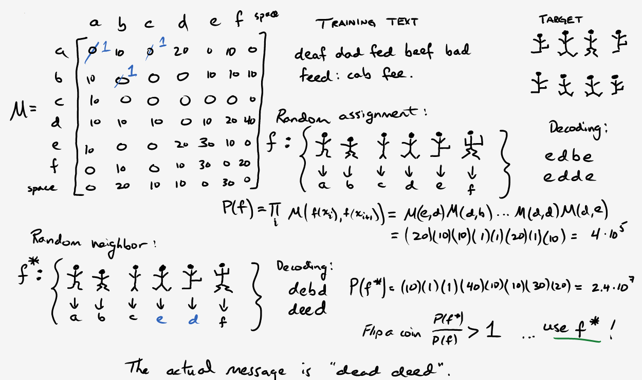
Notice that I multiplied all values by 10 and changed all the 0s to 1s. This is because we’re working with some really limited data. Thus, many letter combinations will have 0 frequency making it hard to compare plausibilities. However, this won’t be a problem with sufficiently long training text.
Now, read the story here and observe how Mr. Holmes cracks the code with a frequency attack and deductive reasoning. Then, come back and take a look at how our algorithmic approach stacks up when decrypting an excerpt from Hound of the Baskervilles. Happy Halloween!
In case you want a challenge, here’s a longer message to decipher below. Fair word of warning: if you blindly assign each new symbol you encounter to a letter, you’re going to run out of letters. The explanation is given in the passage, so I strongly suggest reading it first. Even if you can figure out “the trick” yourself, read the story for fun!