
Last time, we introduced the coffee shop problem and a tool of the data analysis trade, that is gradient descent. This time, we’ll get into the meat of the analysis and finally reveal the winning price and recipe. As a result, there won’t be many interactive elements presenting big new concepts, but there will be plenty code snippets to complete. So without further ado, let’s begin.
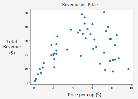
We know how to perform a linear regression, but how do we tackle interesting non-linear patterns like the one between price per cup and total revenue?
Multivariable Gradient Descent
Note that the relationship looks somewhat quadratic. Consequently, we can describe the relationship between price per cup \(x\) and total revenue \(R\) as:
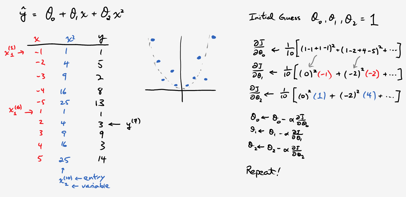
\[R = \theta_0 + \theta_1 x + \theta_2 x^2,\]where \(\theta_0, \theta_1,\) and \(\theta_2\) are parameters. Hopefully this situation sounds familiar; maybe we can use gradient descent in order to determine what those parameters should be. Of course, we only worked with a single variable last time, so we’ll need to generalize to multiple variables. Fortunately, this task is not too difficult and we’ll provide a concrete example shortly. Given a relationship \(\hat{y} = \theta_0 x_0 + \theta_1 x_1 + \theta_2 x_2 + \ldots + \theta_n x_n\) our modified algorithm is:
for \(i\) iterations:
\[\frac{\partial J}{\partial \theta_n} \leftarrow \frac{1}{m} \sum_{i=1}^m (h_\theta(x^{(i)}) - y^{(i)}) x^{(i)}_n \text{ for each variable } 1 \text{ to } n\] \[\theta_n \leftarrow \theta_n - \alpha \frac{\partial J}{\partial \theta_n} \text{ for each variable } 1 \text{ to } n\]
Important notation: the superscript is not an exponent! It refers to a particular data point and the subscript refers to the variable in question. Just in case it’s not clear, when referring to the biases \(n = 0\), we define \(x^{(i)}_0 = 1\) for all \(i\), which ends up being identical to our previous algorithm (try verifying this). Now, in the case of quadratic fitting, we don’t really have two independent variables. Instead, we’ll let \(x_1 = x, x_2 = x^2\) and then go through the usual procedure as illustrated below:
Vectorization
This works fine for a few variables, but what if we’re dealing with tens or hundreds? Performing all these computations and writing out tons of partial derivatives seems impractical. Luckily, there’s a better way with vectorization.
Consider the example above, but written in a slightly different way:
\[\mathbf{X} = \begin{bmatrix} 1 & -1 & 1 \\ 1 & -2 & 4 \\ 1 & -3 & 9 \\ \vdots & \vdots & \vdots \\ 1 & 5 & 25 \end{bmatrix}, \quad \mathbf{y} = \begin{bmatrix} 1 \\ 5 \\ 2 \\ \vdots \\ 14 \end{bmatrix}, \quad \mathbf{\theta} = \begin{bmatrix} 1 \\ 1 \\ 1 \end{bmatrix}.\]In this form, \(\mathbf{X\theta - y}\) calculates all the errors. Special linear algebra commands such as the ones in numpy can perform these matrix operations much more efficiently than doing the equivalent task using loops. It also looks nicer: numpy.dot(X, theta) - y. Try coding a quadratic regression using this knowledge, and then check your implementation with the solution file. It may be helpful write out the psuedocode using matrices first.
Stochastic Gradient Descent
You may have noticed a slight issue. The parabola is concave up, even though it should be flipped upside down. The correct fix would be to increase the learning rate or number of iterations since our cost curve doesn’t seem to have tapered off yet. But for the sake of learning, let’s pretend I didn’t say anything and try a different technique called stochastic gradient descent.
The cost function can be quite messy, and sometimes we can get stuck at local minima (figure a).
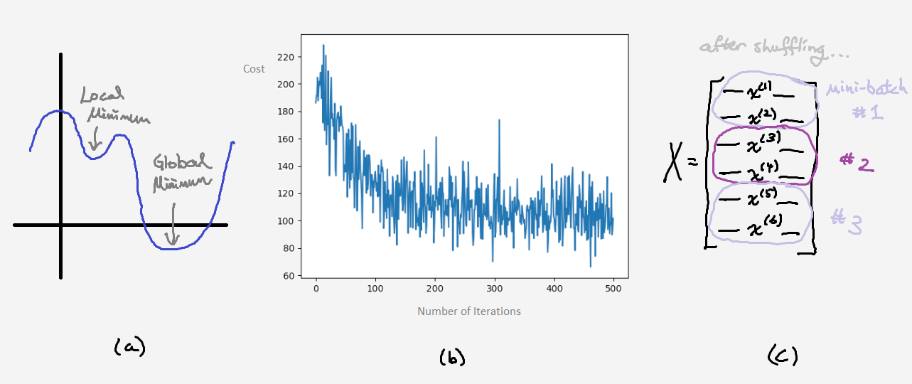
In order to dig ourselves out of this hole, just inject some randomness by training with only one randomly selected data point from the entire set each iteration. Unfortunately, you’ll notice that the cost won’t always decrease each step, and it’s very “noisy” compared to our smooth curves before (figure b). You can also perform mini-batch gradient descent, which is a compromise between this method and our original one. Similar to SGD’s advantages, we begin taking steps downhill without needing to look at the entire dataset, and we can break up huge datasets to fit in RAM if needed (figure c). Additionally, by training on small batches instead of single points, the noise should average out a bit prior to approaching a “good” minimum. Go ahead and try to implement mini-batch gradient descent. The shuffle function may come in particularly handy.
Normalizing the Data
Notice how we already have a better fit using the same learning rate, but with only 500 iterations! However, we can do even better. Let’s return to our initial implementation and increase the learning rate, making sure that \(\alpha\) isn’t too large so that we avoid exploding \(J(\theta)\). Yet, even with \(\alpha\) set as large as possible, our convergence rate still hasn’t been optimized to it’s full potential. In order to make the next breakthrough, we’ll need to rescale our features.
To see why, let’s look at some 3D graphs:
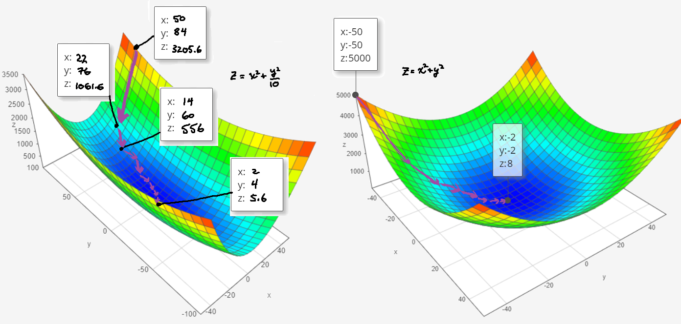
The left plot represents unnormalized features; the axes would be \(x\) and \(x^2\) in our case. Notice how elliptical and elongated the base is. As a result, we will take lots of tiny steps and spend forever inching towards the bottom of the basin when compared to the right side. Furthermore, we may overshoot and form a little zig-zag pattern, especially around the narrow chasm. Contrast this to the “normalized” plot on the right, which takes predictable steps and always points towards the center.
There are a few different ways of rescaling. If you’re familiar with statistics, you could always standardize the data by computing the z-score,
\[z^{(i)} = \frac{x^{(i)}-\mu}{\sigma}\]where \(\mu\) is the mean and \(\sigma\) is the standard deviation. That way, both axes are scaled similarly. However, in our case, we’ll be using max-min normalization which squashes all our values between 0 and 1 inclusive. Specifically,
\[z^{(i)} = \frac{x^{(i)}-\text{min}(x)}{\text{max}(x)-\text{min}(x)}.\]Now, return to our first code example and uncomment out all the relevant normalization lines. How high can you make \(\alpha\) now?
The learning rate can now go up to 1.0 with no problems. Pretty remarkable!
With all these enhancements out of the way, we can finally compute the price point to give us maximum revenue. Just find the vertex by using \(\frac{b}{2a} = \frac{\theta_2}{2 \theta_1}\). WARNING: we’re not finished! This value is normalized. Thus, we’re given \(z\) and we’ll need to work backwards to solve for our price \(x\), which happens to be around $5.20. Okay, now we’re done.
Our Winning Brew
Now that we have our price, all that remains is to formulate the recipe. To do this, we’ll fix the price, collect 50 additional trials, and then run a multivariable regression. Personally, as a non-evil businessman, I would like to take reputation and customer satisfaction into account given that we’ve already tried to maximize our coffee cup price. However, if you plot reputation versus each ingredient…
…the more the better. Unfortunately, maximizing quantity is expensive, so we’ll need to come up with some other reasonable standard. We know that milk is the cheapest ingredient by far ($0.05-$0.10 per cup), so we’ll max out on that (2 cups per serving). Lastly, we’ll make a simplifying assumption. We’ll assign the same variable to both sugar and coffee (since they’re on the same scales), and then solve for this variable in order to make our reputation gain marginally above 0. In math terms,
\[\theta_0 + \theta_{\text{milk}}(2.0 \text{ cups}) + \theta_{\text{coffee }}x + \theta_{\text{sugar }}x > 0 = \Delta\text{Reputation }\]Therefore, rounding up to the nearest tenth, \(x \approx 3.0 \text{ cups}\). That completes the strategy! As for purchasing patterns, I only bought supplies when I was running low and could buy in bulk. After a few days, restocking became a relatively mindless ritual. Now a drum roll for the moment of truth:
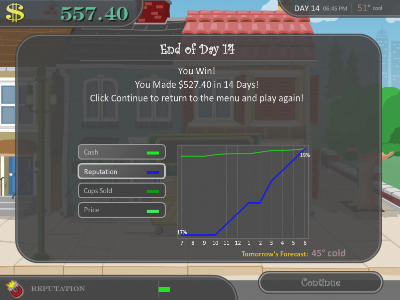
The proof is in the pudding, and clearly, it was good pudding. I recommend trying it out on your own.
P.S. Here’s the product in real life. For the purist, this recipe may sound like an abomination; don’t worry, all I can find is cheap instant coffee. To make it Vietnamese style, substitute sugar with condensed milk. I give it 7/10 for taste.
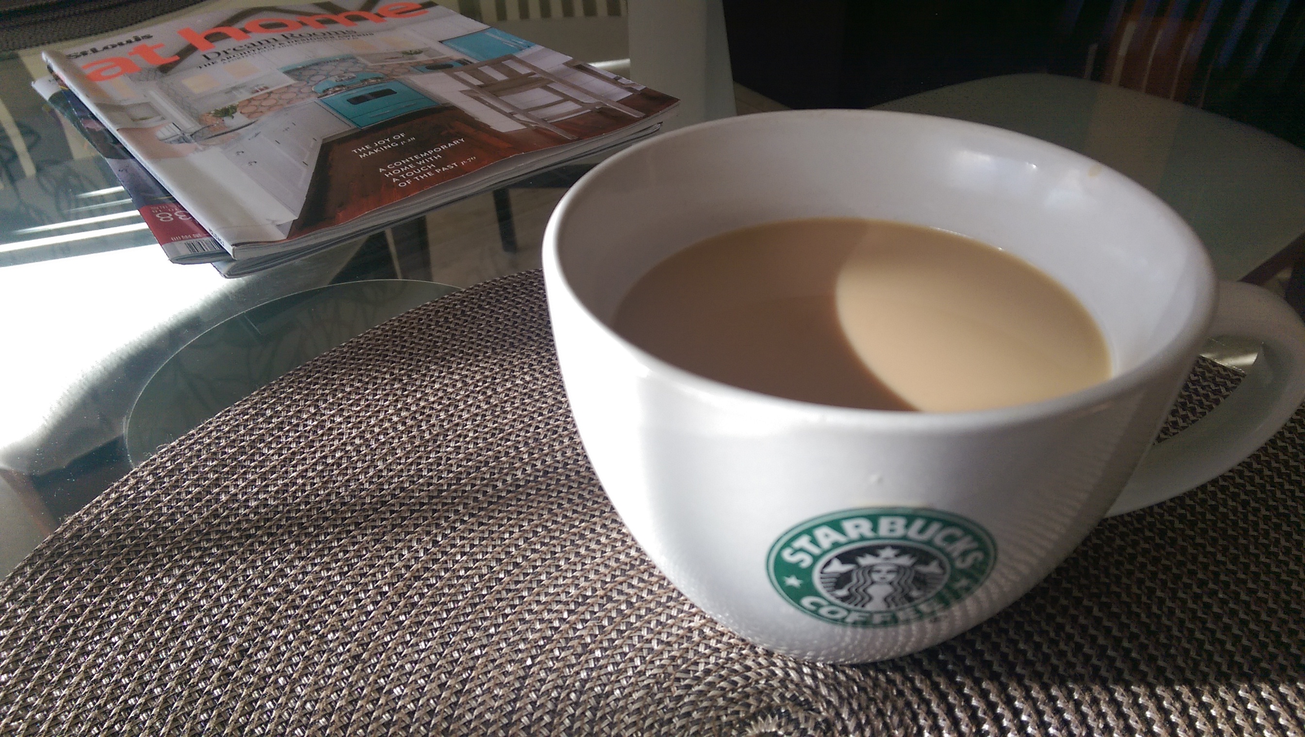
However, when we factor in the Starbucks-inspired price, it’s most certainly a ripoff. Nonetheless, our virtual customers seem to enjoy it, so to each their own. Until next time.