
In middle school, there was a rather popular website kids went to called Cool Math Games (don’t worry, it’s not terribly sketchy). Anyway, I forget the specific details, but I do recall having a bit of “independent time” to work on educational-related things, and one student assured our teacher that the site was indeed, educational. When she found out that learning consisted of Bloons Tower Defense and other nonsense, well…let’s just say that was the end of that. Don’t get the wrong impression; despite this incident, my 6th grade teacher an amazing educator and inspiring individual. Also, Cool Math Games did have some information on mathematics such as an article on counting I tried skimming over at the time. I gave up upon encountering \(n \choose k\), kind of like how I recently struggled through an entire day trying to understand tensors.
So, to make up for the lack of math and to revisit the joys of childhood, I present to you one of my personal favorites: Coffee Shop. Go ahead and give it a whirl. It’s important that you play through at least a few in-game days to make sense of the analysis below (and I apologize in advance for the lack of volume controls; you can always mute the tab if desired).
Our Motivating Question
All right, so what does this have to do with the title? Well, after playing a few rounds last week I thought, “Hmm…what’s the best strategy for maximizing profit?” Since I’ve been spending so much time trying to move into AI and machine learning, I figured this might make for a fun mini data-analysis tutorial that would be different (in an positive way) from other articles out there. In the following sections, I’m going to introduce the experiment and lay out the necessary tools, namely gradient descent. The fine details and substantive analyses will come in part 2.
Some Necessary Simplifications
In order to answer the question above, we’ll need to collect some data. I decided to generate 50 different sets, one for each simulated day. Each set contains 4 random values, chosen over a uniform distribution with appropriate ranges listed below:
| Coffee | Milk | Sugar | Price per cup |
| 0-4 tsps (0.1) | 0-2 cups (0.1) | 0-4 tsps (0.1) | $0.1-$10 (in 0.1 increments) |
Unfortunately, this still leaves plenty of open questions. For instance, temperature has a huge influence on sales. Furthermore, your starting budget will vary depending on how many supplies you purchase. Buy too little and you’ll run out of product, but buy too much and you’ll risk spoiling ingredients. I could record daily profits, though that varies with the price and business reputation, which changes midday. To further complicate matters, purchasing in bulk is cheaper. Yet, anyone who has been to a Costco can attest to the dangers of wholesale shopping. As a result, what do we record, how should we buy supplies, and how do we ensure that measurements can be reasonably benchmarked from day to day?
A time-consuming exercise: if you’re not convinced that we couldn’t have just recorded everything and then trained some complex model (requiring more data), try running 100 days worth of simulations with manually-set random values, record every hour-by-hour detail yourself, and then imagine doing that again when you’re done.
Solution: narrow the scope of our problem, make reasonable assumptions, do a dry run, and then refine and repeat. Specifically, instead of asking our broad question above, let’s only consider day 1. We’ll then transfer that opening-day strategy throughout the remaining two weeks. This provides us with several benefits. First of all, the temperature is always \(51^{\circ}\text{F}\) on the first day and lies between the coldest and warmest days. Secondly, the starting budget is constant at $30.00 and our reputation starts at 0%. Lastly, we’ll spend our entire budget in order to maximize the cups of coffee we can produce. Even if we don’t sell it all, we will need an initial stockpile and most of the supplies will last at least another day.
Admittedly, even this isn’t perfect and I’ll leave you to come up with more reasons why. However, we’ve got to start somewhere, and this seems like a reasonable place. Below, I’ve recorded the reputation and profit for each recipe-price tuple in “data.txt”.
Exploring the Data
Feel free to explore the dataset. The soldout column is indicated with a 1 if we ran out of coffee, which only happens once and appears to be an outlier (in terms of reputation). Consequently, we’re rarely leaving out potential profits, and even then one might argue that this is an acceptable “penalty” in our model since it means we could be charging more.
The “main.py” file is broken into 4 parts: the self-explanatory read_file() function that you can ignore, gradient_descent(), which we’ll get to in a bit, a training block, and a plotting block. In the training block you can find all the data split and stored into appropriate column vectors such as coffee or price. Go ahead and plot some of these variables by modifying the plotting block line ax1.plot(x_variable, y_variable, 'o'), then answer following questions:
- Which two variables seem to be the most strongly correlated? That is, find the two with the closest “straight-line” relationship (ex. height and weight).
Price and Reputation
- Out of the three ingredients, which one appears to be most correlated with reputation?
Milk
- Most of the remaining pairs seem to be either random, or weakly correlated. However, there is one interesting exception…can you identify it?
Price and Revenue. This has a very fascinating relationship, and we'll definitely take a closer look at it in part 2. In the meantime, see if you can come up with an explanation for the scatter plot's distinctive shape.
Linear Regression
Based on the activity, it makes sense to model the relationship between price and reputation with the equation of a line,
\[\hat{y} = \theta_0 + x\theta_1\]where \(\theta_0\) is the y-intercept (bias) and \(\theta_1\) is the slope (weight). However, how do we determine these parameters? If you had a high school experience similar to me, then you may have been taught to plug points into a calculator and magically compute the regression line. This time however, we’ll be doing things from scratch, and trust me, the payoff will be well worth the cost (function).
Suppose we have a model and some points. We can then compute how far off our model’s predicted \(\hat{y}\) is from the real \(y\) by taking a difference. Here’s an example:
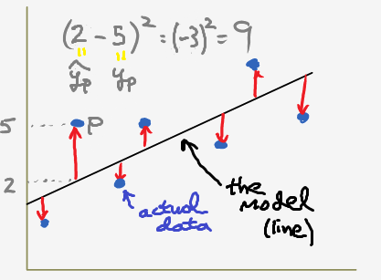
We can then square each of these differences (to get distances) and then take an average of all these “errors”. The resulting quantity is the mean squared error (MSE):
\[MSE = \frac{1}{m} \sum_{i=1}^m (\hat{y_i} - y_i)^2,\]where \(m\) represents the number of training examples. Let’s rewrite this as the following:
\[J(\theta) = \frac{1}{2m} \sum_{i=1}^m (h_\theta(x_i) - y_i)^2.\]Even though this looks a bit strange, it’s the same equation. We’re just going to rename \(J\) to be our cost function, which takes in \(\theta_0\) and \(\theta_1\) as parameters. Similarly, \(\hat{y}\) is going to be a function of \(x\) given some theta parameters. As for that extra 2…you’ll see in moment. All we have to do now is to find the values of theta that minimize our cost function. In other words, take steps in the steepest downhill direction until we reach the bottom. This direction is determined by the gradient, \(\nabla J\) (which involves taking derivatives, or finding slopes along both axes). I thought about \(\LaTeX\)ing the derivation, but opted for an “old(er)-school” way instead:
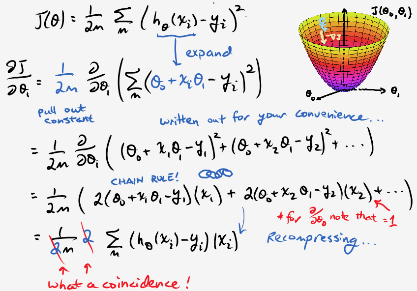
To conclude, here’s the psuedocode for the gradient descent algorithm:
for \(i\) iterations:
\[\frac{\partial J}{\partial\theta_0} \leftarrow \frac{1}{m} \sum_{i=1}^m (h_\theta(x_i) - y_i)\] \[\frac{\partial J}{\partial \theta_1} \leftarrow \frac{1}{m} \sum_{i=1}^m (h_\theta(x_i) - y_i)x_i\] \[\theta_0 \leftarrow \theta_0 - \alpha \frac{\partial J}{\partial\theta_0}\] \[\theta_1 \leftarrow \theta_1 - \alpha \frac{\partial J}{\partial \theta_1}\]
Note that we’ve included a factor \(\alpha\) called the learning rate, which controls how “big” our steps are.
Intuition
To test your understanding, let’s take a short field trip to the French Alps.
Once you’re satisfied with your score, try implementing gradient descent in “main.py” above. Don’t forget to set a few learning rates, plot the cost versus number of iterations (already done for you), and compare the results!
Fortunately, in the time it took to wade through that explanation, our coffee has cooled enough to analyze and I’ve covered all the technical tools needed to do so. Next time, we’ll go into the interesting details and finally reveal a winning strategy (edit: it’s posted!). Along the way, we’ll walk through multivariable regression, stochastic gradient descent, and data standardization. Until then, enjoy this visualization I made encapsulating the main ideas.