
First, let me start off with what this post is not. It is not a thorough discussion into the arguments between Frequentists and Bayesians. With that said, I’ll provide a resource at the end in order to highlight the differences between these two views and give you a reason to care about Bayesian statistics. I delved into this subject myself not too long ago using a course on Coursera that I highly recommend, and this is my attempt to introduce and summarize some of the fundamental ideas.
The Bayesian model is an important paradigm that should be part of an introductory statistics course, yet when I took my university’s equivalent of “Stats 101,” we didn’t even make it to good ol’ NHST (null hypothesis significance testing). Furthermore, a quick Google search doesn’t seem to reveal a lot of “friendly” guides akin to Khan Academy for basic statistics and Paul’s Online Math Notes for calculus. There are some posts, slideshows, and long pdf textbooks that are pretty good, but I find myself glazing through blocks of formality, convincing fooling myself that I understand the concepts, and then losing interest like a kid in high school just waiting for the bell to ring. Ideally, this post will encapsulate the main ideas in a more captivating way.
Bayes’ Theorem
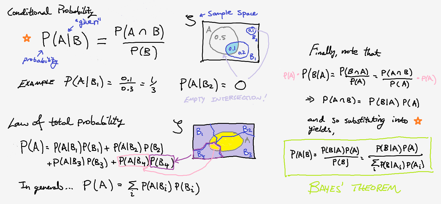
To start our discussion, I’m going to provide a simple derivation of Bayes’ Rule (see image above), which will also serve as a refresher for conditional probability and the law of total probability. Admittedly, it’s not very enlightening for the complete beginner, but it will provide some exposure for the video that follows and hopefully convince you that I didn’t pull anything out of thin air.
With that out of the way, here’s a Veratasium video to introduce the topic and bring up some philosophical points:
In the comments section, several people noted that the choice of prior probability was misleading. Specifically, since the patient had shown symptoms and seen a doctor, it doesn’t seem appropriate to set \(P(\text{having the disease})\) to be the proportion of the entire population with the disease. This is a fair point which we’ll address in the quiz below.
As stated in the video, Bayesian statistics doesn’t tell you about how to pick your prior, and clearly those beliefs will affect your predictions. This might lead you to think that the whole process must be subjective and worthless! Well, not so fast. As this video demonstrates, you’re free to pick whatever prior you’d like, but merely convincing your YouTube audience that the choice is justified can be tricky enough, let alone some scientific committee. Also, keep in mind that although we try to be as consistent and logical as possible, statistics does inherently involve some level of subjectivity from choosing the right model to interpreting the results. Nonetheless, it remains a very powerful tool for making sense of the world around us.
Furthermore, although one has to put some thought into selecting a prior, our beliefs will change as we collect more data. In practice, if there’s enough data, this information will overwhelm any initial biases in our prior. Even in cases where this doesn’t apply, Bayesian statistics provides us the tools to clearly lay out our assumptions and then see how answers depend on those assumptions. Now, if all this still seems too hand-wavy and imprecise at the moment, don’t worry, we’ll make these ideas concrete in the following sections. Before we continue, take some time to make sure you can apply a few basic rules of probability.
Casino Investigator: The Case
Congratulations! Having passed the screening test, you’ve been hired as an investigator for the Missouri Gaming Commission. Your first order of business involves investigating a fraud claim for slot machines at the brand new Atlantic City Casino. According to state law RSMO 313.805(12), “No gambling device shall be set to pay out less than eighty percent of all wagers.” A representative insists that their payout rate is set to 85%, but this contradicts with numerous other reports. As a result, you and I have decided to organize a covert operation.
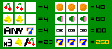
Reputable insider details reveal that it is impossible to obtain three in-a-row, and this appears to be consistent with consumer complaints. However, this doesn’t immediately imply that the payout rate is less than 80%. In order to tackle this question, we’ll need to do some preliminary calculations.
First of all, note that we can only win $4.00 per game given the previous information. In addition, each game costs $1.00. Thus, what is the maximum amount someone can lose per game, on average, in order to comply with regulations?
$0.20 because 0.80/1.00 = 80% of our original bet.
We’ll represent the probability of winning as \(\theta\), and so the probability of losing is \(1 - \theta\). Using the expected value that you calculated above, can you find the smallest (legal) probability of winning?
The player must win 20% of the time (1 out of 5 games on average) since $$-0.20 = 3\theta - 1(1-\theta) \implies \theta = 0.8/4.$$ We multiply by 3 because those are your actual winnings ($4.00 prize - $1.00 to play).
Now that we’ve found \(\theta\), recall that the binomial distribution is an appropriate model since we have \(n\) independent events with two possible outcomes \(x=\{0, 1\}\) and fixed probabilities:
\[\text{Bin}(x; \theta, n) = {n \choose x} \theta^{x} (1-\theta)^{n-x}\]Let’s say we play a single game. How likely is it that we lose?
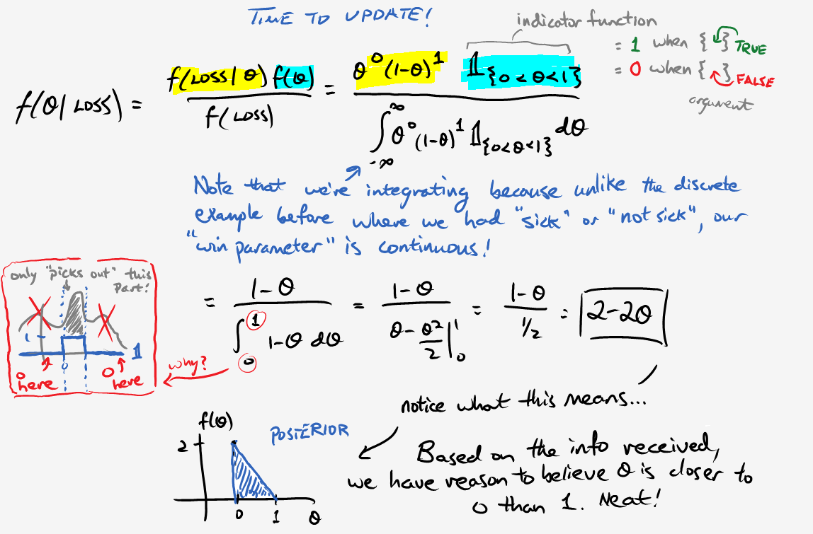
This boils down to the Bernoulli distribution (special case when n=1) where x represents a win. $$\theta^{0} (1-\theta)^{1-0} = 1 - \theta = 1 - 0.2 = 0.8,$$ which is just a complicated way of finding something we already knew. The next one won't be nearly as trivial.
If we play 5 games, how likely is it that we win less than 4 games?
This is the same as taking 1 - P(winning 4 or more games). Working out the details, $$P(x \geq 4) = {5 \choose 4} \theta^4 (1-\theta)^{5-4} + {5 \choose 0} \theta^5 (1-\theta)^{5-5} = 0.00672$$ Thus, the answer is 1 - 0.00672 = 0.99328.
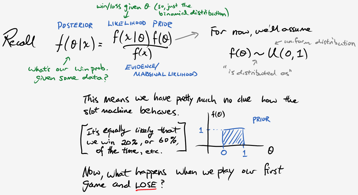
We’re ready to bring Bayes back into the picture. The section below will provide some insight into how we can use the data in order hone in on what the probability of winning for the slot machine actually is.
Repeat the same procedure above, this time considering a win. (I promise it’s not as painful as it seems.)
$$f(\theta \vert \text{Win}) = \frac{\theta}{\int_0^1 \theta d\theta} = \frac{\theta}{1/2} = 2\theta$$
Unfortunately, even after all that work, we’re still left with some issues. For example, we’re pretty sure that the slot machine has a payout rate of 85% or less (which corresponds to a win rate of 20% or more), but our chosen prior doesn’t reflect that knowledge. Also, if we have to keep integrating after every game, your operation will take ages and I will go insane. Fortunately, we’re going to resolve these complications in one fell swoop; behold, the beta distribution.
\[\text{Beta}(\alpha,\beta) = \frac{\Gamma(\alpha+\beta)}{\Gamma(\alpha) \Gamma(\beta)} \theta^{\alpha-1} (1-\theta)^{\beta-1}\]A few important notes: it looks intimidating, but upon closer inspection, it’s fairly similar to a binomial distribution. That weird looking \(\Gamma\) is the Gamma function, and it’s just a generalization of the factorial. Careful though, because \(\Gamma(n+1) = n!\). Also, the mean of this distribution is \(\frac{\alpha}{\alpha + \beta}\).
Go ahead and play around with this distribution to get a sense of what it looks like (part 1 only). Hold \(\alpha\) constant and vary \(\beta\), then swap. What do you notice? What happens if you change \(\alpha\) and \(\beta\) together, maintaining the same ratio?
Progress at last! We finally have a way of selecting a more detailed description of our beliefs. Now onto actually calculating the posterior:
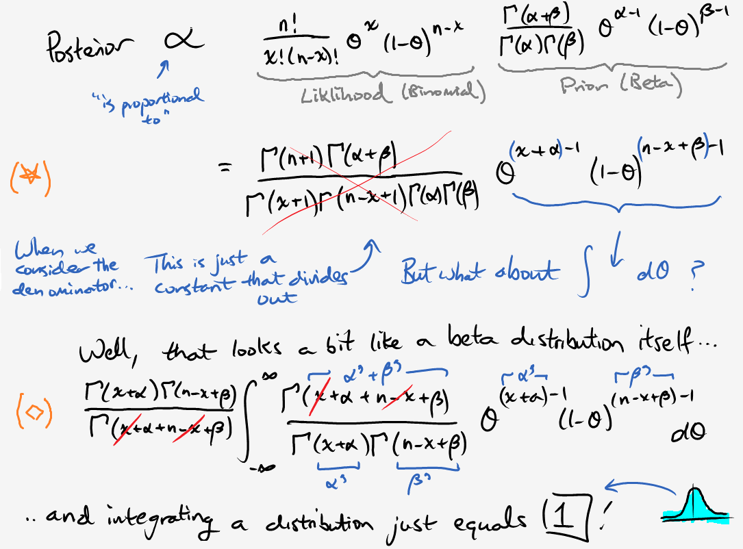
Consequently, we see that
\[f(\theta \vert x) = \frac{(\star)}{(\diamond)} = \frac{\Gamma(n+\alpha+\beta)}{\Gamma(\alpha+x)\Gamma(\beta+n-x)} \theta^{x+\alpha-1} (1-\theta)^{n-x+\beta-1},\]and so if our prior \(f(\theta) \sim \text{Beta}(\alpha, \beta)\), then our posterior \(f(\theta \vert x) \sim \text{Beta}(\alpha + x, \beta + n-x).\) Notice that the prior and posterior are both beta distributions. Thus, we say that the beta distribution is a conjugate prior for the binomial distribution. More interestingly, notice that in order to update our beliefs, we simply add the number of wins to \(\alpha\) and the number of losses to \(\beta\). The new mean is:
\[\frac{\alpha+x}{n+\beta+\alpha} = \overbrace{\frac{\alpha+\beta}{n+\beta+\alpha}}^\text{weight}\underbrace{\Big(\frac{\alpha}{\alpha+\beta}\Big)}_\text{prior mean} + \overbrace{\frac{n}{n+\beta+\alpha}}^\text{other weight}\underbrace{\Big(\frac{x}{n}\Big)}_\text{data mean},\]or just a weighted sum between the prior mean and the sample mean (look carefully)! In summary, we can interpret \(\alpha\) as “prior wins”, \(\beta\) as “prior losses”, and \(\alpha + \beta\) as our effective prior sample size. If \(\alpha + \beta \gg n\), then our prior beliefs will dominate and data will only “nudge” the posterior. On the contrary, if \(\alpha + \beta \ll n\), data will be our primary influencer regardless of the prior.
Casino Investigator: Fieldwork
We’re now ready to begin collecting data. First, choose an appropriate prior and be sure that you’re able to justify this decision. Keep in mind that you will be playing 200 rounds (and I’m already playing, so I’ll do 300). The casino hasn’t been around for long, so we haven’t compiled any historical data. The only information we have comes from the casino representative and consumer complaints. I would suggest giving little weight to either side (to avoid casino reps claiming foul), and then let the data speak for itself.
Once you’ve made a choice, head over to the slots. Feel free to use the utility below in order to tally your results:
Wins: 0 |
||
|
Total: 0 |
Losses: 0 |
Now, update your prior then plot the likelihood and posterior (part 2). Try overlaying all three graphs and view the results. Do they make sense? Is it what you expected? All right, time to reconvene. Here are my findings: wins: 44, losses: 256. Go ahead and update your results once more and then report the final posterior distribution.
Casino Investigator: Analysis
We can now use our posterior distribution in order to make predictions about what we think the value of \(\theta\) is by constructing a 90% credible interval, which seems like a fair standard for deciding whether to escalate things further. Specifically, let’s find the highest posterior density interval (HPD), or the smallest range of \(\theta\) values such that we envelop 90% of the probability mass like so:
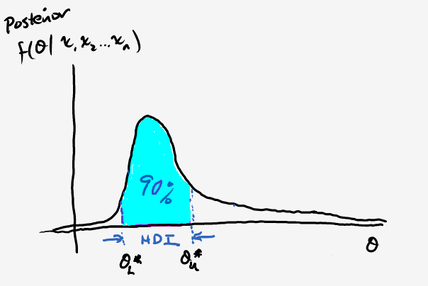
This is an analogue to the confidence interval, but they have very different interpretations (this is a great read). In order to do so, we’ll be using the scipy.stats module. Take a look at the documentation (scroll down to the modules), and then complete part 3 of the code snippet above.
What do you notice?
Conclusion
\(\theta=0.2\) is outside our HPD and we certainly have reason to be suspicious, especially when you consider some of the statistics for other casinos. Take a look at the public report for August 2017. Most of the electronic gaming machines have a payout of nearly 90% or more.
Fortunately, with your findings, a spot inspection was approved to analyze the slot machine’s programming; the probability of winning was set below 20% (do double-check the exact value yourself). Busted! Ironically, even without the hefty fine, Atlantic City Casino would have been but a fictitious memory anyway. With such low-stake and low-payoff games, they could attract neither the frequent risk-taker nor the casual newcomer. It’s reputation plummeted alongside its profits, and with that came it’s final chapter, Chapter 13.